


Deriving LVR six ways
and estimating it 10 ways

I included derivations and calculations in the footnotes of my last post, but I omitted some steps and assumptions that might make the explanation difficult to follow. This is intended to provide a clearer exposition. By downloading this spreadsheet, you can see that the nine different estimates (presented after the derivation) are equal.
A simple example helps us understand the nature of convexity costs (aka LVR, gamma cost, theta). Convexity refers to any nonlinear payout, such as a call option where the payoff is max[0, StockPrice – Strike]. If the initial value of a stock is 100.00, and its future value will be either 101.0 or 99.00 next period, the payout for a call option will be
Up: +1.0 (101 – 100)
Down: 0 (call payout has a minimum of 0)
The expected value of the call here is the probability (50%) times +1.0, which is +0.5. However, the payout is risky in that it is 0 or +1. Risk can be eliminated via a hedge, specifically, a short 0.5 stock position that generates the pnl 0.5*(100 – futureStockPrice) in the next period. With a short stock position, we have the portfolio payout.
Up: +0.5 (call payout +1 and short stock pnl of -0.5)
Down: +0.5 (call payout of 0 and short stock pnl of +0.5)
A hedged convex position can turn a risky pnl into a riskless one by amortizing the expected pnl into a certain return, like an interest rate, and this is what LVR or theta do. In the above example, the convexity was positive, so we are creating a positive return, but if it were negative—like an LP position—it would be a negative return.
Using the amortized cost of a hedged position with non-zero convexity is more efficient than using the actual payout because positions are generally held for several weeks. The actual IL for an LP uses a single price path over that period, which is one observation. This has the same expected value as a delta-hedged position, and the delta-hedged position will generate many more independent observations. The hedged subperiod hedged returns are independent because asset returns are independent from period to period, which is a reasonable assumption given otherwise we could all get rich mean-reverting or trend-following daily returns. Many independent observations benefit from the Law of Large Numbers, generating estimates with smaller standard errors. Thus, by estimating the LP’s IL, assuming they are delta-hedging, we can better approximate a best-practice LP experience and generate a more efficient IL.
Constant product pool primitives
The following constant product AMM assumptions underly the various estimate derivations.
I will use ETH and USD as my example tokens, as I find this easier to intuit than x and y. USDC is clearly the numeraire asset (i.e., the price refers to ETH's price, which is USD). One can replace either with BTC, PEPE, etc.

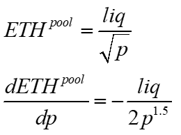
Given the price p, the market value of ETH and USD in the pool are identical

Using the above equations, we can substitute ETH with USD/p and USD with ETH*p to derive the amount of USD and ETH in the pool, given the pool's current price and liquidity.
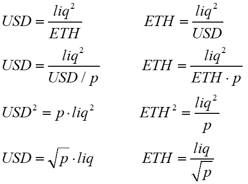
This leads to formulas for determining the change in tokens as a function of the change in price and vice versa.
These equations are used in the following derivations of convexity costs. Different derivations help develop intuition about these costs. Even though they look different, they all lead to the same expected value (i.e., mean), so whatever resonates is valid.
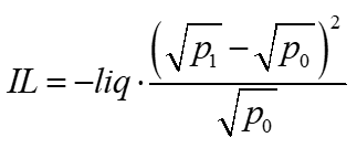
Derivation #1: impermanent loss
The problem with impermanent loss is that it is often referred to as an LP's loss moving from a particular initial price to subsequent prices. For example, an LP with an initial pool price of 100 will see its IL rise when it rises to 102 but then fall when it returns to 100. This generates much confusion, especially the idea that this cost is impermanent and therefore irrelevant.
A better way to measure this is sequentially, such as when the price moves from 100 to 102, and then use 102 and 100 as the next starting and ending price, respectively.
While it is true that the unhedged LP would experience a zero IL when the price goes from 100 to 102 and back to 100, this is just one path. It is best to assume every price change in your sample is hedged and, thus, generates a fresh IL. Over time, the expected and actual ILs will converge via the law of large numbers, so with 30+ daily data points, you can get a reasonable estimate.
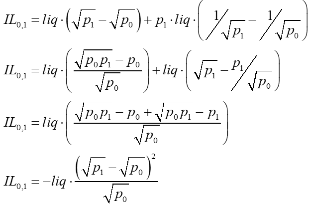
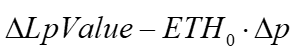
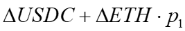
The basic formula for impermanent loss from time 0 to time 1 is the value of the LP's position compared to the value of the LP's initial deposit to the pool (his original 'hold-on-for-dear-life' portfolio).
Impermanent Loss = LpValue – Hodl
This can be rewritten as

Rearranging and relabeling the difference from time 0 to 1 as the pool’s delta, we get

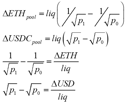
Given the pool primitives on delta ETH and USD above, we can substitute for ETH and USD changes to make them functions of liquidity, and the starting and ending prices.
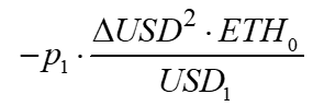
Derivation #2: arbitrage profit
The LP is on the other side of each trade with the AMM. Excluding fees and gas means the LP's gain is a trader's loss and vice versa; it's a zero-sum game. Further, the math in AMMs allows us to take the net amounts of coins A and B in a pool over a period instead of calculating this for each trade. For example, a sequence where a trader buys 1.0 ETH, sells 2.0 ETH, and buys 3.0 ETH, has the same effect as just buying 2.0 ETH. Thus, we can anthropomorphize the trader's net buys and sells over time and treat them as if they were simply one trader, one transaction.
The basic pnl for the trader is the amount he bought times the current price minus the fill price.
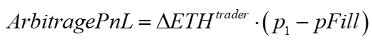
The AMM's effective trade price, or fill price, is the ratio of USD traded over the amount of ETH traded. This ratio equals the geometric mean of our sample period's initial and ending prices.
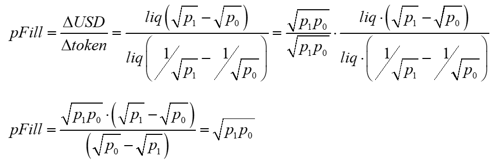
We can also substitute for how the change in the arbitrageur's ETH corresponds to the pool's liquidity and starting and ending prices.
Substituting these into the arbitrage pnl, we get the familiar result, except here, it is positive.

This equals the negative of IL, which makes sense given this is a zero-sum game; the arbitrageur's PnL is the negative of the LP's IL. The big trick here is to calculate this for a pool over daily observations, using mean liquidity and a starting and ending price. Calculating for specific LP positions with different starting times makes them hard to interpret, like averaging the net return over a month by averaging the total return of several stocks with different start times and durations.
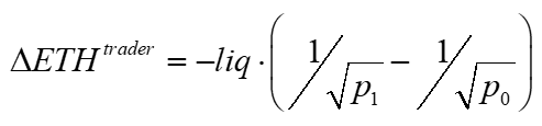
Derivation #3: delta hedged LP pnl
Assume the LP hedges his asset position with the other asset. For example, an LP in the USD-ETH pool hedges his long ETH position by shorting ETH with USD. The LP’s ETH pool position is his 'delta,' the derivative of his position with respect to a change in the ETH price. To hedge, he shorts his ETH pool position on, say, Binance, trading at the initial and ending price.
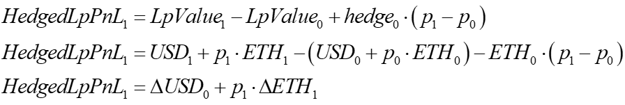
This was already solved in the impermanent loss calculation in Dervitation #1. Its solution is thus the same:
Derivation #4: expected convexity cost
A Taylor expansion of the LP's expected value shows the expected value of a concave function as its current value plus the term with the second derivative.
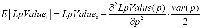
This implies the LP's value change absent fees is equal to the term on the right

The variance of p is in units, so we take the volatility, which is in percent, square it, and multiply it by the variance.
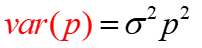
[For example, with 80% volatility and a price of 50, we have Var(p) = 0.8^2 *50^2 = 1600]
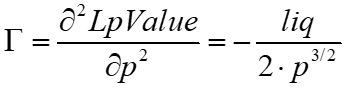
Given

We can solve for the second derivative of LpValue
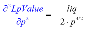
Substituting for these values gives the following, which is negative because the LP's position has negative convexity.

Derivation #5: theta from Black-Scholes
A portfolio with nonlinear derivative V is hedged in continuous time, making it riskless.
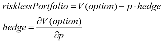
In equilibrium, the options decay, or theta, plus the convexity adjustment should equal the portfolio's cost times the riskless rate.
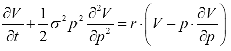
If interest rates are zero, the time decay or theta is equal to the negative of the messy term with a second derivative, denoted gamma. This is because, in equilibrium, the expected value of this position is zero; the time decay (theta) has to offset the convexity cost in equilibrium. The essence of an option is that this term is non-zero, reflecting the curvature or convexity in the portfolio's value.
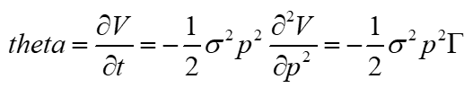
Gamma, the second derivative of the LP position value, was derived in Derivation#4 above:
Thus, substituting for gamma generates the following cost that needs to be offset by fees for the LP to have zero profits. The Black-Scholes theta is positive because it represents how much the LPs should earn to offset this cost.

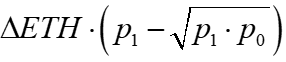
Derivation #6: LVR
Milionis, Moallemi, Roughgarden, and Zhang (2022)'s primary motivation is to view LPs as adversely selected. For example, assume the AMM price is p0, but p1 on Binance. Arbitrageurs will trade against the stale AMM. The arb's fill price—the geometric mean of p0 and p1—will be lower than p1 when p1>p0, and higher than p1 when p1<p0. The interpretation is that the poor LP gets bad fills for all the arb trades. If the LP knew the Binance price, they would sell for 101, but the logic of the AMM makes them sell for an average of ~100.5. Thus, the 0.5 profit for the arbitrageur is a loss for the LPs. This was the motivation for derivation #2 above.
While the above story is their usual motivation, the authors also note this is the same as looking at the delta-hedged returns of the LP (derivation #3 above). However, they name their convexity cost function after comparing the LP with a portfolio replicating its position changes on a centralized exchange (ie, at the true price). This synthetic LP position they call a ‘rebalancing portfolio,’ and the difference between LP and rebalancing portfolio they call loss vs. rebalancing, or LVR. These are all equivalent, so it's not wrong, but it's odd they named it after their own least common story used to motivate it.
The AMM trades via a formula that forces its fill price to be the average of the transaction's initial and ending prices. The rebalancing portfolio trades the identical amount at the arbitrageur’s price, which is the Binance price. The difference in value of these trades is LVR.

Let’s define the Binance price as being some amount r different than the AMM's pre-trade price, presenting an arbitrage opportunity.
AMM initial price = p
AMM end price = Binance price = p*(1+r)
The AMM’s fill or trade price will be the geometric mean of its initial and final price, or sqrt(p*p*(1+r)). The profit per ETH traded is thus:

For small r, as in continuous time, the mispricing is r/2

This gives us
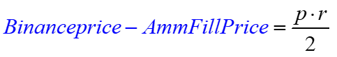
To get ETH to the Pool, they use the derivative of the pool's ETH position with respect to price, times the change in price, which we assume to be p*r (the initial AMM price times the return difference to the Binance price).
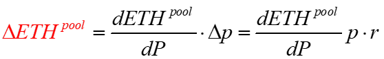
Given a pool's ETH function, we can calculate its derivative
So we can substitute these into our original LVR function and generate our result

r2 is just the variance term, so we have
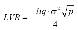
Here, LVR is the cost to the LPs.
Calculation
In general, there are two ways to calculate this. One method is to use the pool's liquidity, starting and ending price. As these are equivalent to changes in pool tokens (i.e., without fees), they generate several identical functions depending on whether one uses the change in tokens, or liquidity and price changes. Below, time 0 is the starting time, the initial AMM price and token amounts, and time 1 refers to the end time prices or token amounts. All the ETH and USD change amounts exclude fees.
The basic IL calculation
LPvalue - Hodl
The delta-hedged LP. The LP's initial delta is his pool ETH position, ETH0, so he shorts that somewhere
The net pool cashflow can be use the net pool token changes (excluding fees).
Thorchain's SLIP fee was designed to eliminate the LP's IL on a trade. I don’t know the derivation, but if you substitute for these tokens with liquidity and prices, you get the above equations. The more the merrier.
The arbitrageur's profit (change in ETH from the pool's perspective)
Given the equivalence of ETH and USD changes to changes in prices and liquidity, the above are all equal to the following
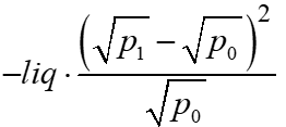
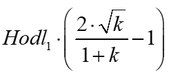
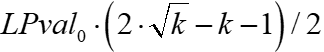
Defining k=p1/p0, we can write #6 as both #7 and #8
TopazBlue’s formula. Here, the initial LP position is valued at the end-of-period price.
I’ve seen this, but I forgot where. It’s just a rearrangement of the above.
If variance=ln(p1/p0), the LVR/theta formula is equivalent to to above within a couple of basis points

See the attached spreadsheet to see them applied
Method #2:
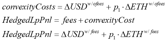
Uniswap’s event logs include fees. Thus, we can use these to estimate the Pool’s pnl assuming the LP collective delta hedged as
Fees are taken in both tokens usually, but we can just take the sum of the absolute value of all the numeraire token changes and multiply this by the fee, as over day it will be sufficiently close to the USD value of the ETH fees.
It is my favorite because no 'liquidity' is needed, which can sometimes be challenging to obtain. Second, this is a straightforward measure of the pool’s true profitability, abstracting from the LP’s long position in the tokens. As mentioned in my prior post, the impact of the LP’s long token position on LP profitability is a distraction.
To generate the convexity costs, we take the Hedged LP pnl and subtract the fees, which can be estimated from the gross USD traded in the period times the fee.

Thus we can rearrange the above to back out the implicit convexity costs, given the Hedged Lp pnl that comes from the net token changes that include fees.

Volatility and liquidity vary, and as any simple technique will discretize the data, this will generate noise in our estimates. There is no way around this problem. If we used data from each trade within each tick, this would benchmark against high-frequency prices that are not true prices due to both the bid-ask on CEXes with their CLOBs and the fee on Dexes. This true price mismeasurement creates the bias where 5-minute markouts generate lower ILs than 4-hour markouts and, worse still, 24-hour markouts. These are obviously the result of bias because if they were real, we would see momentum in intra-day crypto returns, which we would not.
I use daily estimates, which generate comparable convexity cost estimates using either of the above methods when averaged over a month. Here are the two estimates for data on 15 pools since 2021 using the monthly average daily convexity costs (320 pairs of observations).
