

Egorov's IL Elimination AMM
Doubles? Eliminates? Same thing.

Last week, Curve’s Michael Egorov presented a white paper outlining Yield Basis, an AMM that proposes eliminating impermanent loss (IL) through a dynamic leveraging strategy. He raised $5M for this venture back in February, so he has had enough time and resources to present his mechanism as well as it can be presented.
If a new crypto mechanism is superficially plausible, the KPIs are mercenary influencers and consultants, combined with a rewards program that subsidizes initial users with the new protocol tokens. It’s all about marketing. For new AMM designs, the game is rigged. Everyone knows AMMs are flawed due to impermanent loss (IL) dominating fee revenue for capital-efficient AMMs (see here), yet no AMM or well-known third-party provides LPs or investors any information on their pools’ IL. This allows all the AMMs to post LP returns of 40% or higher, which is inconsistent with the universal acknowledgment that net LP profits are generally negative.

These misleading LP gross returns are rarely challenged unless there’s a catastrophe, such as what happened to Fluid this May or Thorchain this January. Anything that requires an understanding of gamma will be incomprehensible to the cryptocurrency enthusiasts who invest in these new, worthless projects. Thus, one crypto Twitter posted his bullish take on Yield Basis under the banner TL:DR, which is a reasonable assumption for what Yield Basis investors will think of the following analysis: too long, won’t read.
Without fully understanding the proposed mechanism, I was instantly skeptical because the method focuses purely on adjusting the USD liability. If it were possible to eliminate LP gamma by adjusting one’s debt, this implies someone could sell options with zero theta. The Linear Pricing Rule is a basic result that says the price of any asset or payoff is a linear function of its future cash flows. That is, the presence or absence of other positions in a portfolio does not affect the value of any asset within a portfolio. This implies that if you can eliminate a loss via a hedge or trading rule, then the hedge or trading rule has a positive return.
Suppose a short option position has a return of 0%, due to its offsetting theta and gamma drift. If one could eliminate the gamma drift by adjusting one’s debt, this USD rebalancing strategy would have a positive return; people could generate profit by dynamically borrowing and lending USD. It’s absurd. Everyone would be able to turn their long gold/Apple/yen position into a squared gold/Apple/yen position, without paying an option premium.
Egorov tweeted that the folks at Yield Basis love all feedback, especially criticism. However, he warns critics that
-you should really understand the protocol before making public statements against it (we’re surrounded by some of the brightest minds in Web3 who’ve already approved the concept).
Egorov’s step-by-step logic appears superficially solid, and it took me a while to figure out where the flawed assumption was hidden. I can see why many of the brightest minds in Web3 think they can get away with it, just as they continue to present LP returns without accounting for the LP’s expense, IL. Given the success of Fartcoin, or Thorchain’s Lenders program, crypto developers are funded by people who have generated lots of wealth for themselves, creating useless and even value-destroying programs.
Egorov’s argument goes like this (see this tweet). The LP’s value is a linear function of the square root of price, which generates the negative convexity.
Assume the investor leverages an LP position using leverage L, generating a USD debt of d.
The investor’s net position would then be the value of the LP position minus his debt. This translates into the notional value of his asset position divided by L.
He then takes the total derivative of eq(3a), V*=V-d, assuming d is constant, divides both sides by V*, and substitutes V* on the RHS with V/L.
This implies that the percent change in the investor’s levered LP position is equal to the leverage amount times the percent change in the LP position. Integrating both sides leads to
This log equation implies that V* is proportional to V raised to the power L
Given V is a function of the square root of price, if we choose L=2, we square V, which is a linear function of the square root of p. Thus, V* becomes linear in the price.
A linear function has gamma equal to zero, so there is no gamma drift, no IL. Or, as Egorov argues in this tweet, the above equation implies
Thus, argues DeFi_Cheeta, an initial levered LP position with a value of $100,000 increases to $200,000 when the BTC price jumps from $50,000 to $100,000.
Note the inconsistency that V*=V/L in eq(3), but V* is proportional to VL in eq(6). The problem is that he treats d as a constant in eq(3a), but then d as a function of V in eq(3b). Going from eq. (4) to Eq. (5) assumes L is constant, though if true, the percent change in levered LP position only equals the percent change in price at the initial price.
What I think he’s trying to capture is that if a position has a power payoff.
Take the natural log of both sides to get
Differentiate both sides with respect to p
Multiply both sides by p
Which leads to
The left-hand side shows the percent change in the value of the power payoff asset, where the exponent is 1/L, equals 1/L times the percentage change in price; a 1% change in price generates a 1/L% change in value for such an asset. Given the LP position value is linear in p^(1/2), a 1% change in price generates a 0.5% change in LP value. If you lever that 2 times, the 1% change in price generates a 1.0% change in the levered position value. So, you can get to the result that the levered position’s percent change is increased so that it is locally equal to the underlying price percent change, but that does not extrapolate to imply gamma is zero.
Levering an LP position two times by borrowing USD doubles the delta, and more importantly, the gamma. That means it doubles the expected IL, rather than eliminating it.
If the BTC price doubles from 50,000 to 100,000, the only way the value of his levered LP position could get to 200,000 would be for his debt to decrease from $100 to $ 82 K. That’s inconsistent with debt defined as a linear function of the gross LP position value.
The issue he neglects is that if you are changing your debt as the value of the asset changes, this implies cash flows you cannot exclude from your analysis. A debt reduction of 10 requires an outflow of 10; a debt increase of 10 implies an inflow of 10. The comparative statics of the LP position’s balance sheet, excluding these cash flows, reflect only a part of LP's profitability. If we add the debt changes to the change in the LP’s net position value, we can see that it doubles the gamma (column (6)).
USD Values and PnL for Base and 2x Levered LP Position
initial BTC price = $50,000, Base Liquidity = 223.6
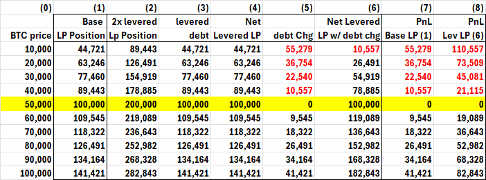
Column(4) above mirrors the base unlevered position. If you assume the debt in column (3) is constant at each new price, you do get the percent change of this value equal to the percent change in price. However, column (4) does not generate any real leverage, as shown by its equivalence with column (1).
For the levered position in column (6), the delta and gamma are double that of the base position in column (1). This can be seen by noting the PnL of the base and levered positions in columns (7) and (8), where the levered position PnL is double that of the base PnL, as expected.
Another way to see how this approach is off-target is to note that the HODL position, like the initial LP position, also has a derivative of one-half the price % change at LP inception. HODL’s value is linear in price: ETH0*p+USD0. The key to HODL’s linearity is that its delta does not change, not that HODL’s percent change equals the price's percent change at every price.