


Fees and LP Profitability
and why auctions, fillPrice=end-of-trade-price, don't work

[Thorchain’s] Slip fee is arguably the most profound innovation in the Thorchain system, as its ability to reduce impermanent loss burden on LPs is significantly greater than in the fixed-rate fee model.
Thorchain’s (TC’s) variable slippage or 'slip' fee is proportional to trade impact. A trade that pushes the price up by 0.2% generates a fill price 0.1% higher than the initial pre-trade price, and the slip fee would add another 0.1%. TC promoted their slip fee as a significant improvement, and all initial research reports touted this as a distinct competitive advantage over it competitors (MultiCoin, Delphi Digital, Gauntlet).
Understanding why the slip fee, or any fee that charges an end-of-trade price, does not eliminate impermanent loss helps one understand automated market makers (AMMs) generally and AMM arb behavior more specifically.
Given the lack of empirical data when TC created its AMM in 2021, the slip fee was a plausible improvement over a fixed-fee AMM. The benefit was reaping extra revenue from ignorant or impatient traders, and the cost was the effect of traders gaming their fee by splitting it up and distrust by ignorant and impatient traders. Ultimately, the slip fee’s efficacy is an empirical question. Someone should have been monitoring its performance as real data became available, but no one inside or outside TC did that.
Understanding how the slip fee would probably work involves technical details beyond most people's interest. In mature industries, executives don’t need to know the details because there’s a large community of experts with practical knowledge who can monitor and manage technical processes and hold each other accountable. Thus, executives can trust that technical issues they do not understand are being managed efficiently. In infant industries like AMMs, protocol executives can only rely on themselves, so they must be familiar with the essential details.
Even if you do not care about the primary metrics of AMM performance, the following details are instructive about the sort of details that matter. Further, assuming arbs will compete until they generate zero profits is clearly absurd, so one must understand how the absurdity is avoided.
Background: IL and Arbitrageur Profits
The liquidity provider’s (LP's) impermanent loss (IL) is the flip side of arbitrageur profits. To see this, consider if we abstracted from retail traders and assumed the pool had a single arbitrage trader and zero fees. The arb's profit would equal the LP gamma expense in that case. This should be intuitive because this is a zero-sum trade between the arb and the passive LPs represented by the pool. Thus
If we add in the fees paid by the arbs, this is still a zero-sum game, so the net arb PnL after fees will equal the LP’s net PnL: fees minus IL.
[Appendix: arb profits and IL for a fuller explanation1 ]
Perfectly Competitive Arbitrageurs
A fee rate increasing with trade size motivates arbitragers to split their trades. In the limit, the arbs send trades as small as possible to minimize their fee expense, eliminating any potential benefit of the slip fee mechanism [Appendix: Splitting Trades to minimize the slip fee2]. However, TC's special sauce was that, as it runs on its own Cosmos blockchain, it would apply a block sequencing rule that requires transactions with the highest fee trades first. If the true price is 1% away from the current price, an arb breaking his entire trade into 10 trades would be front-run by the aggressive arb who broke up his trade into just 5 trades. This reasoning continues until one arb makes a trade pushing the price 1.0%, making zero profit, and the LP suffers no IL.
Another application of this reasoning is the frequent batch auction approach, where arbs engage in repeated auctions every block (Moallemi and Robinson, 2024). In a standard auction equilibrium, the arbs compete until their profit is zero. However, perfect competition in the flat fee case should also lead to zero arbitrage profits as arbs jump on incremental AMM mispricings that sum to nothing.
Even those promoting the idea that slip fees or auctions can pull all the profit back from arbitrageurs do not think it would actually be true. Everyone knows businesses need to profit, or they will exit. But then you must ask, 'What limiting principle allows the competing arbs to maintain positive profits?'
Economic theory has little to say about the nature of equilibrium profits, that is, profits above the standard CAPM returns on capital. For AMM arbs, the high-frequency nature of their strategy, combined with daily hedging or rebalancing, generates a zero CAPM beta, and so, the risk-free rate of return.
An obvious adjustment would be to incorporate the arb’s costs, as capturing DEX mispricing takes a considerable investment in APIs, pricing algorithms, etc. However, at the moment of an arb’s decision to trade, these can all be considered sunk costs, irrelevant to the arb’s trade decision, which has effectively a zero marginal cost. In standard economic theory, there is no stable equilibrium in industries facing zero marginal costs and positive fixed costs.
The best theories about economic profits involve barriers to entry and collusion. Collusion requires a small set of players because the costs of monitoring and the benefits of cheating increase exponentially in the number of players. The barriers can be regulatory, such as the duopoly of Standard&Poor's and Moody's, or railroads that have become natural monopolies due to the modern political impossibility of laying new tracks.
In market making, the barrier involves the hardware and software required to respond quickly to price anomalies. The winner-takes-all nature of arbitrage rewards only those who are first, and a power-law distribution in proficiencies tends to produce a small set of potential winners. This generates a barrier to entry competitors who cannot see and react to these mispricings at the scale needed to make arbitrage possible.
With zero fees, the arbitrageur makes the same profit whether he trades every second or once at the end of each day. This is because if the initial and ending prices were the same, the arb's net tokens traded and ending price would be the same. The arb trading each block would have a much higher gross amount of tokens traded, but there are no transaction costs in this example, so that would not matter. With fees, the arb maximizes his profit by waiting as long as possible so that the CEX-DEX mispricing edge is greatest. If an asset moves 5.0% in a day and the fee is 0.30%, his ideal trade places an order at the end of the day, capturing an edge of 4.70%. If he trades when every 0.31% deviation arises, he will trade more frequently but with a lower edge. The latter will have lower net profits, apparent in the LP gamma recapture equation derived below.
Competition forces the arbs to operate on a sufficiently small edge that only a select few can sustainably play the game. However, given that small set, at some point, they no longer compete on edge. Instead, they focus on speed and selectivity instead of price competition that whittles the edge and profits on each trade to zero. The marginal benefit of beating another arb if their orders collide in a block becomes second-order. This allows an equilibrium where the arbs generate a net profit after fees. [Arb Equilibrium for Non-Zero Edge] 3
The arb accounts are easy to identify if we look at actual pool data, as the top five accounts generate at least 50% of the pool volume. The average price impact for these accounts is relatively consistent among these dominant arb accounts. Commonly, an arb will make consistently sized trades all day, say $1000, which implies a consistent price impact on an AMM.
Fixed Fee Arb Objective
The arbs pay the fee to the LPs, so the greater the fees the arb pays, the greater the amount of the LP's IL that is offset. However, the degree to which the fee covers the LP's total IL varies based on the fee rate and what I will call the ‘edge,’ the price movement generated by the arb (ie, end-of-trade vs. pre-trade price).
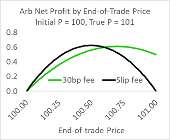
To see this, consider the chart below for a case where the fee is 30 bps and the edge is 70 bps. The arb's optimal end-of-trade pool price is 100.7, because, at that point, his incremental fill price, including fees, will be the true price, 101.0 (100.70 + 30 bp fee). At that point, his marginal profit of 0.30 equals his marginal cost of 0.30.
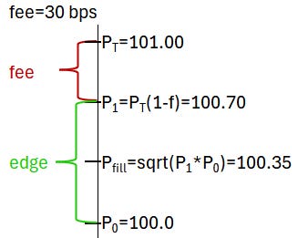
The arb’s net profit after fees is just the value of his position at the new true price minus the fill price and the fees he paid.
Break up the true price into the fee and edge components (eg, fee is 0.003 and edge is 0.007)
On an AMM, his fill price is the geometric mean of his trade’s initial and ending price. His end-of-trade price is his initial price adjusted by the edge.
Substituting these generates the arb's net profit as a function of the edge.
For an edge less than 1%, we can substitute ‘1+edge/2’ for ‘sqrt(1+edge).’ Ignoring the edge*fee term as second-order gives us
The ETH traded, ΔE, given how much the arb intends to push the price, the trade’s edge. Given constant product AMM math, ΔE can be replaced by liquidity and the edge.
Substituting this gives
We can calculate his daily profitability by multiplying the profitability per trade by the daily number of trades he makes. An arb trade is triggered when the price is at least 'fee + edge' away from the current price. If there were no fee, the number of times his edge would trigger a trade would be the total variance over a day (eg, n*variancePerBlock) divided by the edge squared.
The above is a standard result in stochastic processes. With no fee, when the arb trades, the problem restarts as it was initially. The fee complicates this because the new trigger barriers are asymmetric once an arbitrage trade is made. At that point, the AMM price will be closer to the CEX price on one side and further on the other.
For example, assume the price starts at 100.0, the edge is 0.2, and the fee is 0.1. A price move up or down 0.3 triggers an arbitrage trade. In the example below, when the CEX price rises to the red cell at 100.3, the new post-trade AMM price would be 100.2.
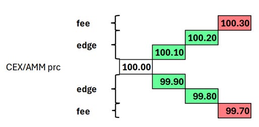
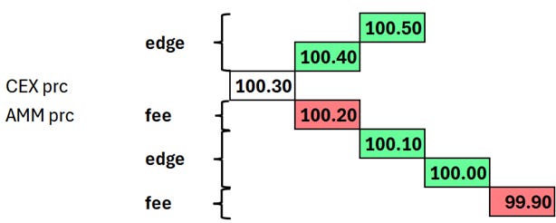
After the arbitrage trade, the boundaries triggering an arb trade are asymmetric. In the chart below, the CEX price is 100.3, but the AMM price is only 100.2 because it stopped at the CEX price minus the fee. Thus, continuing the CEX price’s earlier move requires only two steps up to generate the 0.3 trigger (100.5-100.2 = 0.3); the reverting move has to first double-back over the fee buffer, then proceed through the edge, and then move by the fee amount (99.90 - 100.2= -0.3).
The probability of hitting a boundary decreases exponentially by distance, so moving up 0.2 or down 0.4 has a significantly higher probability than moving 0.3 in either direction. The simple formula for hitting a barrier does not directly apply, as it presumes symmetric barriers. The precise number can be calculated directly in a lattice, but the expression is the sum of a series of combinatoric functions multiplied by probabilities, which does not aid intuition. However, the following formula works well as a concise approximation.4 It takes the base case of the symmetric barriers and multiplies it by a ratio with the fee over the edge in the numerator.
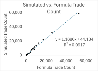
I simulated an arb trading strategy 10k times using various fees and edges for a fixed AMM liquidity over a day where the total volatility was 10%, and there were 260k periods, so each step had an average 2 basis point movement. I then applied fees and edge combinations ranging from 0 to 100 basis points in steps of 10 for a total number of 121 combinations (e.g., {10, 30}, {100, 60}).
Multiplying the number of trades and the profit per trade, we get the following result for the arbitrageur's profit after fees for a given edge and fee.
Note that the LP's gamma expense (aka lvr) is the leftmost ratio.
Arb profits are LP losses, given the zero-sum nature of the pool. So the LP's percentage of IL mitigated by the arb fees, as a percentage of IL, is
The above notes that if arbProfit is zero, the LP recaptures all of his IL via the arb’s fees; if the arb’s profit is maximized at the entire IL, then the LP recaptures zero of his IL. Substituting into the above, we get.
If edge > 0 and fee = 0, the LP gamma recapture rate is zero, which makes sense because the LP has no revenue and only his gamma expense. If edge = 0 and fee >0, the LP gamma recapture is 100% (technically, the left-hand term equals zero as the edge approaches zero from +infinity. The zero-edge case is often mentioned as the result of perfect competition in continuous time. If arbs eliminate their profit after fees, given the zero-sum game, it implies that the LPs capture all of the gross arb profit as fee revenue.
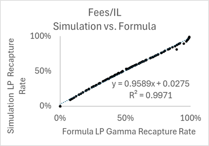
I simulated arb behavior 10k times for 121 combinations of fees and edges over a day with a 10% move and trades every 300 milliseconds. This is like the simulation mentioned above about the trade count. I then averaged the pool's fees divided by the day's gamma expense (aka IL) and compared it to this formula. The results show that the LP gamma recapture formula above is an excellent approximation.
The fixed fee for pools is usually 5 or 30 basis points. The edge applied by arbs will vary based on the blockchain latency, gas costs, and pool liquidity. Further, the state of MEV power on various blockchains varies, and the costs arbs must pay for various transactions could be significant. A pool arb's average edge can be observed by looking at the handful of addresses generating 50% to 80% of an AMM's trade volume. Depending on the pool, their trade price impact on their trades will be relatively consistent, between 3 and 12 bps.
For a given edge, the effect of the fee on the LP's recapture rate is a concave function that implies diminishing marginal returns to a higher fee. A higher edge lowers the LP's gamma recapture rate. We should expect the edge to be higher in higher fee pools because otherwise, the arbs would not make a sufficient profit; for low fee pools, the equilibrium arb edge will be lower because otherwise, it would be too profitable to arb, and then there would be too many active arbs, which would make their collusive equilibrium untenable.
The Slip-Fee Arb Objective
In the fixed fee case, the arbs respond whenever the CEX-AMM price exceeds 'fee + edge.' The slip fee is dependent on the size of the edge they apply, which, if a function of the fee, generates endless recursion. However, it turns out there is a simple solution if we assume there is some edge the abs consistently apply.
The arb's profit and costs are functions of the true price, pT, and the end-of-trade price the AMM uses to apply the slip fee. Note that the slip fee is just the arb's profit if his end-of-trade price is the true price (the AMM has no oracle).
Solving for the optimal target price p1 generates a cubic equation without a closed-form solution. However, the p1 that optimizes net profit equals the mean of p0 and pT. [Appendix: Deriving optimal slip fee target price] 5
We can see this by looking at the net profits for an arb whose initial starting price is 100 and the true price is 101.00. We then calculate the arb's total profit, assuming his end-of-trade price is between 100.00 and 101.00. With a 30 bp flat fee, the arb's maximum profit price is 100.70, 30 bps below the true price. The arb facing the slip fee maximizes his profit by targeting his end-of-trade price at the middle of the initial AMM price and the true price, 100.50.
If the slip-fee arbs move halfway to the true price, we can model the profitability of the arbs. If slip fee arbs come to an equilibrium where they employ a similar ‘edge’, this edge would be the half-way point between the AMM and the true price. We must reinterpret some terms to fit this into the above model applied to the fixed fee case. First, we define 'edge' as how much the arb moves the price on a trade, though with the slip fee, this does not contain the arb’s profit but rather his all-in cost. What corresponds to the ‘fee’ in the above fixed-fee model here corresponds to the slip fee arb’s profit, as he stops here, just as the fixed-fee arb stopped at the edge of the fee.

Given that the edge and fee are equivalent, we can label the fee as the edge in our formula. We can then solve for the LP gamma recapture rate just as we did for the fixed-fee LPs. [see derivation in appendix]6 The answer is.
Given that the LP's gamma expense is the term on the LHS, the slip-fee LP's fee recapture rate from arb trading is
Interestingly, the slip-fee arb's profit and the implied LP gamma recapture rate are independent of the arb's edge. It doesn't matter whether the arbs collude to trade only when the edge is 1.0% or compete down to a 3 bps edge; the effect is the same. 33% is a significantly lower LP IL recapture rate than for reasonable edge estimates applied to 5 bp flat fee pools, which would be 67% given a generous 5 bp edge. The slip fee fails as a mechanism for offsetting IL if we assume arbs are not engaging in perfect competition but instead are applying standard refinements—an equilibrium edge—once they eliminate all but a handful of competitors.
Don’t Care! What’s the Point?
TC never monitored the LP IL, which supposedly benefited significantly from their signature slip fee. It would have been helpful marketing if they had data to support their fee’s advantage. If anyone bothered to look, they would have noticed that TC arbs would often average 3 bp fees over months, significantly lower than the lowest-fee AMMs. Further, from the start of TC data until the minimum 6 bp fee was instituted in August 2024, arbs were often making several small trades within the same block, contrary to the story that competition would prevent this tactic.
Most people are ignorant about most things, as we have different priorities, limited time, and too many complicated subjects to ponder. However, when businesses do not monitor whether their signature innovations work, nor does anyone who wrote about this distinctive advantage, it suggests none of these groups are serious about the long-term viability of what they are doing (and that crypto consultants are paid shills). In 2023, TC moved to streaming swaps that effectively eliminated the hefty fees from imprudently large orders, presumably because the cost of annoying traders was greater than their enhanced fees from imprudent trades. By then, no one cared about the slip fees, as they had served their purpose.
The problem with impermanent loss is that it is often referred to as an LP's loss over a specific period. With hindsight, it is easy to see whether the put or call was worthless or valuable, like looking at who one should have bet on in the last big game. The key is to get as many independent data points as possible, and a particular period for a particular token is essentially one data point.
While the expected IL over a year is the same as the 365 daily expected ILs, the latter's advantage is that you have 365 independent samples instead of 1. As token returns are uncorrelated day-to-day, the daily hedged returns generate 365 observations.
The basic formula for impermanent loss from an initial time 0 to an ending time 1 is the value of the LP's position compared to the value of the LP's initial deposit to the pool (his original 'hold-on-for-dear life' portfolio).
Rearranging we get
or
In the above, ΔUSD is from the pool's perspective, so positive means the pool gains USD. It abstracts from the initial token amounts as if they do not matter, like assuming the initial LP position is hedged.
By definition, on average, noise traders have zero net demand for each token (aka white noise), implying the net token changes are due to arb token changes. This motivates the opposite view: if we multiply the above by -1, we have the arb's profit over that period, as the opposite of the pool's net token changes is the arb's net token changes.
Given the pool primitives on delta ETH and USD above, we can derive the same equation as the function of the arb's net pnl, where we multiply the amount of ETH bought times the end-of-period price minus the arb's cost per token, pFill.
The amount paid by the arb for ETH will equal the pool's USD balance change.
Which implies
There are many ways to intuit and mathematically generate IL and, by extension, the gamma expense. One can also apply pool identities to show this equals a different formulation, such as
This gives comfort to the fact that this matches another standard metric for IL.
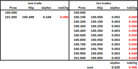
Impermanent loss increases with the square of the price impact, and a slip fee mirrors the IL. Thus, moving a price 20 bps costs 4 times as much as moving a price 10 bps. If all arbitrage trades are small, with price impact 2-10 bps above the fee, the fee generated will be significantly lower than the total IL over the sequence of trades. To see this, consider in the table below. On the left, a single trade moves the price 100 bps, and the trader pays a 0.249 USD slip fee, which is 0.25% of the trade amount (0.062/0.25 = 0.25% price change. In the second scenario, given the same AMM liquidity, the trader makes 10 sequential trades of one-tenth the size, and the total sum of fees for those trades is 0.025 USD, which is one-tenth the amount. As the slip fee increases non linearly, the arb's dominant strategy is to trade small. This can be further split up so the fee becomes infinitesimal.
At some level, arbs focus on latency, not price competition with their competitors, because that's a winnable game. Many investments that help arbs that do not involve price: RPC access, NVMe SSD storage, Field-Programmable Gate Arrays, Kernel-bypass NICs, etc.
A powerlaw in proficiency generates a handful of arbs that can trade at the lowest latency. They are playing a repeated game where one arb is usually making a trade when no one else wants to. The large retail trades that generate MEV interest for front-running and sandwich attacks generate a lot of attention, but this is a different game and is irrelevant to LP IL. Arbs are targeting mispricings under 10 bps, often under 5. The parochial differences in their 'true price' aggregation model will generate random discrepancies across arbs. In practice, arbs do not compete within blocks.
The arb has to consider two extremes in an AMM with a fee. In one, he assumes no competition, and his best strategy is to wait as long as possible so the fee as a percentage of his gross profit is the smallest. In the other extreme, he eliminates his competitors’ profits, as well as his own, by aggressively trading on every infinitesimal profit opportunity. Why this is so is shown above, but at this point, assume it is true.
Let us define four gradations of aggressiveness in our arb trader’s strategy. In one extreme, he chooses the least competitive trading strategy that maximizes his profits, assuming he has no competitors. On the other hand, he can be considered a profit blocker, preventing other arbs and himself from generating a net profit (i.e., after fees).
Max-Prof: Profit from trade targeting a large trade
Aggressive: Profit from trade targeting modest-sized trade
More aggressive: Profit from small trades
Zero-Prof: making an almost infinite number of super-small trades
Assuming the arbs split profits when trading the same strategy (probabilistically getting half the profit on average), as they both generate the same slippage (per the slip fee sequencer rules), the winning arb is chosen randomly. If one arb is more aggressive than the other arb, by generating a larger trade, they can then dominate arb trading and leave their competitors with nothing. However, at that point, his competitor would make a zero profit and could improve his profit by applying a more aggressive trading tactic. This generates the following normal-form game.

Payoffs to trader A on left of comma, for trader B on right
While there are only 4 possibilities above, this is just meant to show the basic pattern. AMMs are not constrained to minimum tick sizes, so there are an almost limitless number of potential pricing tactics (target 1 bp below the true price, 0.99 bps, etc). If traders A and B competed in a finite sequence of games, one can see how they would gravitate towards the bottom right corner equilibrium where both make near zero profit. That is the Nash equilibrium.
In real life, arbs often trade without competition due to random issues. For example, one arb may have a portfolio that is maxed out in their position on a token, so they cannot buy more. More commonly, the 2-10 bp opportunities are at the edge of detection, given randomness in their API feeds and the model they apply to decoct the ‘true’ price out of these feeds. When arbs trade without competition, their payoffs are trivial in that they do not depend on what the other player is doing. However, it is useful to present them this way to see how they add up. Below, we see a normal-form game when an arb trades without competition. The Nash equilibrium here is in the upper left, the opposite of when the arb competed.

Making the conservative assumption that DEX arbs compete on half of their trades (usually much less), their expected profit payoff per trade takes the average of the payoffs in the above matrices. This shows a unique equilibrium in the upper left where they trade as if they were not competing.

An arb could focus on the parasitic strategy of just targeting the successful arbs and immediately post a more aggressive trade that would generate a higher slip fee and get executed first. However, once the other arbs see what is happening, they could punish him in many ways. For example, if one arb acquires an excess inventory of ETH, as is natural, he expects to pay at least 5-10 basis points to sell these on another exchange. Instead, given that he expects to pay to unload the ETH anyway, he could place costly sell orders on the AMM merely to bait the price-jumping arb to make unprofitable trades. It would cost him nothing, but he would punish the penny-jumping arb who thinks these exit trades are arbitrage trades. Implementing a rule that presumes an opportunity solely based on other’s trades is dangerous because these other traders can generate manipulative counter-measures.
The key to maintaining a colluding edge is that they primarily compete on latency, risk management, and their model of distilling a true price given several, if not thousands, of potentially relevant data points. The Coinbase and Binance prices are relevant, but so is the futures price for US stocks, which is correlated with these prices. The set of prices relevant to Bitcoin’s true price is large and undefined.
The fastest traders with the best true price model will dominate almost everyone. The handful who can compete then play a repeated game with a handful of competitors. Given the second-order benefit from outcompeting other arbs and the zero-profit endgame, one can see why arbs do not engage in price competition as if they were bidding on assets in an auction.
an even better approximation is
For my purposes, the extra precision does not change any of my points. In practice, a lattice could calculate an even better estimate.
The arb's net profit maximization problem is
Thorchain has its own derivation of the slip fee,
This has nine other identical formulations, representing the IL on a trade. We can substitute the one with the same use of liquidity, initial and end-of-trade price; we can create an objective function that allows us to solve for the optimal end-of-trade target price by the arb.
Taking the derivative of this equation with respect to p1 and setting it equal to zero finds the arb's profit-maximizing target end-of-trade price, p1. Solving for p1 with gradient descent quickly finds the solution: the mean of p0 and pt.
This allows us to define the true price in this strategy as
The slip-free trader’s all-in cost, which includes the trade impact and fee, is thus
Using the earlier formula of netProfitPerTrade, substituting for the true price and the fill price (including fee), we have
Given ΔE defined above, we have
or
Using the formula for the number of trades above, noting that in this case, edge = fee, we have
Multiplying the profPerTrade times the number of trades gives
which simplifies to