

The Impact of AMM Fees on Arbitrage Trade Fee Revenue
The Impact of AMM Fees on Arbitrage Trade Fee Revenue
there's a formula!
Gross arbitrage profits are independent of fees
Arb trade volume decreases with fee
LP revenue from arbitrage trading is strictly increasing in the fee
Most papers on AMM fees and arb trading are 'not even wrong,' despite Milionis, Moallemi, and Roughgarden's (2023) generous assertion that 'there is a rich literature on constant function market makers.' For example, Evans, Angeris, and Chitra (2021) find the optimal fee to be 'near zero,' a silly result (see below). The only paper I found that generated an empirical estimate of arbitrage trading was Heimbach, Pahari, and Schertenleib (2024), who use heuristics to estimate at least 30% of AMM trading comes from arbitrage, but they do not distinguish how pool fees affect arbitrage trading, and this is just a lower bound.
Most of these papers suggest lower latency would mitigate arbitrage profitability, presumably benefiting LPs. Lower gas fees and lower latency chains have been around for a couple of years, and LPs there are not more profitable than the slow Ethereum mainnet, so models or intuition generating that implication are profoundly misspecified.
The issue is that all functioning AMMs have arbitrage traders driven by profits to update the price on pools. The are net costly to AMMs, but they perform an essential service, and hopefully non-arbitrage traders exist in sufficient volume to offset the expense generated by the arb traders.
The basic LP profitability is its revenue, generated by trades, and its costs, which come from adverse selection inherent to all market makers. I call the expense convexity cost because it derives from the convexity of the LP position, which has been studied for 50 years in option pricing theory. However, it is also known as impermanent loss (IL) or Loss vs. Rebalancing (LvR), and these generally refer to the same thing.
LP net profits = TotVolume * fee – convexity costs
Convexity costs are solely affected by the underlying asset's volatility and the LP convexity and are independent of hedging tactics. An excellent hedge can amortize this expense into a fixed cost but cannot lower it.
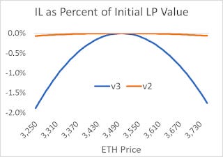
Capital-efficient AMMs using restricted ranges were introduced in Uniswap v3, and they leverage an LP's position within the targeted range. The range below shows the Impermanent Loss for two LP positions, one an unrestricted (v2) range, the other with the same liquidity but with a range of $3250 and $3750. The curvature in these two lines is the definition of negative convexity. These two LP positions have the same level of convexity (i.e., the same gamma), generating the same USD expense, but as this v2 range uses only 3.5% of the capital as the v2 range, it generates 1/0.035, or 28 times more convexity cost than the v2 range as a percent of capital. This is how the more popular capital-efficient AMMs elevated convexity costs from a curiosity to an existential threat.
AMM LP Negative Convexity
Decentralized AMMs are a thousand times slower than the major exchanges and will always and forever follow centralized exchange prices. The convexity cost is generated from a given level of liquidity, price, and volatility. This is one equation; note there is nothing about arbitrageurs or latency.
LP convexity cost = variance * liquidity * sqrt(p) / 4
An important identity when examining arbitrageur profitability is that the LP's convexity cost mirrors the arbitrageurs' profit.
Gross Arbitrage Profit = LP convexity cost
The gross prefix implies pre-fees, which is an important distinction, as the arb pays a fee to the LP, but we will address that later. While one can see an earlier blog post for a mathematical explanation, the intuition is straightforward: as this is a zero-sum game, the LP's convexity cost is someone else's gain. We can anthropomorphize the net token changes over a period as the arbitrageur's trades because, by definition, 'noise' traders are random white noise and have a zero net impact on token changes over longer durations and price movements.
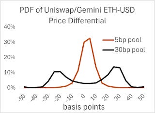
Empirically, active AMM pools are relatively efficient, with their AMM price within the fee of the centralized exchange (CEX) price (which generally are within 5 bps worldwide). The chart below shows how the AMM price differs from the CEX price over the past 6 months for the 5 and 30-bp ETH-USD pools, where I took the CEX price and compared it to the AMM pool price over the next 30 seconds. This implies the AMM arbs are active, and we can presume they apply a standard arbitrage algorithm.
Data from 2023-3/2024
We can ignore the second-order effect of AMM price deviations to the CEX prices and look at how the price of ETH (or whatever token) changes to see how this affects the arbitrageur's profit. At the end of a day the AMM price will vary by +/- fee over the CEX or 'true' price, but this effect washes out to insignificance.1
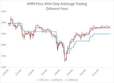
The effect of fees on arbitrage trade volume can be intuited by noting that arbitrageurs do not trade to lose money. They will only push the AMM price up to within 5 bps of the true price: (1 – fee) *p; or down to (1 + fee)*p when the AMM price is higher. Within that bound, the arbitrageurs are absent. For example, here's a price graph for a 6-hour period, and we presume there are only arbitrage traders affecting prices for pools with 5 and 30 bp fees. Note both AMM prices are less squiggly than the true price, and the blue 30bp fee price moves less frequently than the red 5bp fee price. This is why arbitrage trade volume decreases with the fee. It's like looking at a coastline with different granularity, where the coastline using 50 km units is greater than that same coastline approximated with 100 km units (while in theory, the coastline is infinite, in practice, the granularity of sand keeps it finite).
Any arb algorithm has a minimal profit buffer, as no one wants to implement a trade that will generate a one satoshi profit after paying the AMM fee. If one tries to lock in a profit, the other leg of the arb will cost at least 5 bps (including fee, spread, and price impact). Most likely, arbs do not hedge each AMM trade, but the amortized cost of hedging still includes a cost. An arb has to profit after expenses, and the AMM fee is just one of them.
Fluctuating gas costs and latency also create uncertainty. Ethereum mainchain blocks are constructed every 12 seconds, but even the lowest latency chains for a decentralized AMM are at best 300 milliseconds compared to microseconds for a CEX, and the disappearance of a resting bid could move the CEX price by 5 basis points. It is prudent to add leeway for this epistemic risk.
As the arb's trade directly impacts the AMM price, he moves the price up to the CEX price, which is adjusted by the fee to a target price.
If (pCEX/pAMM – 1) > (fee + min_edge)
Sell until pAMM = pCEX*(1 + fee)
If (pCEX/pAMM – 1) < - (fee + min_edge)
Buy until pAMM = pCEX*(1 - fee)
Effect of the edge
For example, consider this scenario where the fee is 5 bps, and the minimum edge is 5 basis points (edge is in a percent of the price, whereas 'minimum profit' in hummingbot is in dollars)
pCEX = 100.10
pAMM = 100.00
fee = 5 bp
edge = 5 bp
pool liquidity = 1e6
The arb would buy until pAMM = 100.05
pfill = sqrt(100.0*100.05)=100.025
USD sent to pool = liq*(sqrt(100.05) – sqrt(100.0)) = 2499.69
USD paid in fees = 0.05% * liq*(sqrt(100.05) – sqrt(100.0)) = 1.25
ETH bought = - 1e6*(1/sqrt(100.05) - 1/sqrt(100)) = 24.99
Gross Arb Profit = LP convexity cost = ETHbought*(pCEX – pfill)
ETHbought*(pCEX – pfill) = 24.99*(100.10 – 100.025) = 1.87
net arb profit = Gross Profit – LP fees = 1.87 – 1.25 = 0.62
LP fees/LP convexity cost = 1.25/1.89 = 0.67
In this example, the arb paid 67% of the gross profit. As gross arbitrage profits equal the LP's convexity costs, the LP covers only 67% of her convexity costs.
There is another minor issue with latency or the discrete nature of trade times and pricing. Since the rule is to arb trade if the pAMM is above or below a threshold, the price that triggers a trade on average will be above the cutoff. For example, if the annualized volatility of ETH is 60%, its volatility every 12 seconds is 0.04%. Add to this that the CEX trade price data comes in from bid to ask, generating a 0.05% standard error. In real life, as opposed to continuous time, these effects create at least 1 bp price difference. When measuring its effects, we should add this to the explicit edge number above to get the effective edge number because the average discrepancy drives the results.
The edge in any arb trade would be a combination of the minimum required edge plus the edge generated by waiting until the signal was greater than this. For example, if the arb bot waits until the edge is 5 basis points, it will probably be 7 or 8 basis points when the trade is initiated. The general formula estimates the effect of the edge on arb trade revenue as a percent of the LP's convexity costs:
ArbTradeRevenue/convexity costs = fee/(fee + edge/2)
The edge is divided by two because the fill price will be approximately halfway between the edge price and the CEX price adjusted for the fee. In the example above, the fee was 5 bps and the edge 5, so 5/(5+5/2), which is 67%. This allows us to see how LP arb trading fees cover the LP's cost as a function of fees and the edge. With an edge near zero, any fee would maximize arb trading fee revenue, including the case highlighted by Evans et al. In real life, trading for a few wei every zeptosecond is not a helpful ideal.
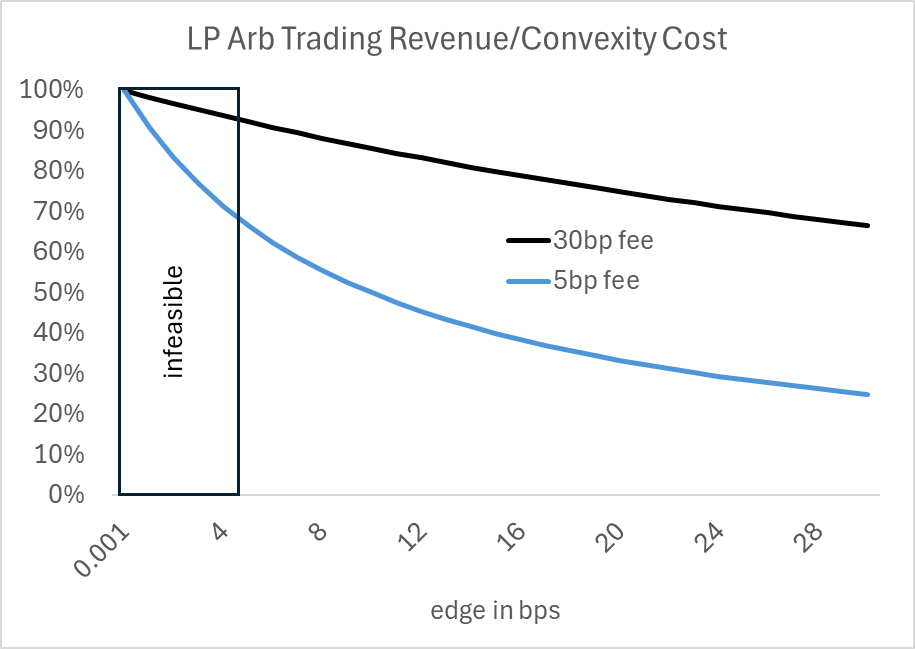
Note that the higher fee curve is always above the lower one, highlighting that arb trading volume falls by more than the fee. That is, for a given edge, the product of arb trade volume times the fee decreases as the fee decreases; volume rises by less than the fee falls.
One way to intuit this is to note that hedging frequency does not affect convexity costs. We know gross arbitrage profit in continuous time does not depend on the trade frequency. If the buffer creates a wedge where only 67% of gross profits are paid on each little trade, over time, total fees are only 67% of gross profits.
We can estimate this applying a Monte Carlo simulation on downsampled ETH data, applying the above arbitrage formula using a minimum edge of 5 basis points. As the per-minute volatility is about 5 basis points, the effective edge is around 10 basis points, as we effectively censor data outside of the tail. We can then calculate the amount of arbitrage trades on an ETH-USD pool using the sum of the change in the square root of ETH price on all the trades each day, as 'sqrt(ptarget) – sqrt(pAMM)' represents the amount of USD traded for one unit of liquidity. If we normalize each day by the square root of the ETH price, we can average the daily data from 1/1/23 through 3/1/24. The results are in the table below:
Monte Carlo Simulation on Minute Downsampled ETH-USD data
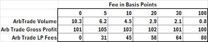
Arbitrage trading fees are just the volume traded times the fee. Note the gross arbitrage profit is approximately constant, as expected. Thus, fee revenue is strictly increased in fees as a percentage of convexity costs. Arbitrage trading LP fees will never exceed LP convexity costs because arbitrageurs need to make at least zero profit, and gross arbitrage profits equal convexity costs.
We can also apply the daily arb trading volume per unit of liquidity using 5 and 30 basis point fees and an edge of 5 basis points to the daily liquidity for several ETH-USD pools.
Arb volume estimated using the above arb bot algorithm applied to Arb Trade Volume estimated from minute-downsampled data, multiplied by daily pool liquidity
Data from 1/1/23 through 3/1/24
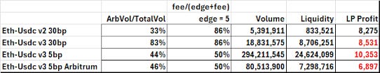
Here, we see the v3 pools all losing money over the period. While the 5bp pools have three times as much noise trading (1 – arb trading vol/totalVolume), the above chart shows why they were just as bad as the ETH-USD v3 30 bp pool. The ETH-USDC v2 pool, however, generated LP profits because it has relatively more noise trading, and its arb trading volume covers more convexity costs than the low-fee pools.
The ETH-USD v2 pool has consistently made money, both before and after the arrival of the v3 pools in May 2021. The relatively significant amount of noise trading on the more expensive ETH-USD v2 pool could result from the competitive aspect of front-ends that route trades to the AMM with the best price. If one AMM has a fee of 5 bps, the other 30, the odds the 30 bp pool will be picked would be only 0.5*5/30, or 8% of the time (explanation left as an exercise for the reader). Given the size of the 5bp pools relative to the v2 30bp pools, this would be sufficient to generate the noise trading volume.
A stupid conclusion would be to assume that higher fees are necessarily better. As arb trading revenue will never exceed convexity costs, these pools need noise traders and are affected by fees. Lower fees will generate more noise trading. One can see this by expanding the algebra:
LP net profits = totvolume * fee – convexity costs
LP net profits = (noise volume + ArbTradingVolume) * fee – convexity costs
LP net profits = noise volume * fee + arbvolume * fee – convexity costs
LP net profits = noise volume * fee + fee/(fee+edge/2)* convexity costs – convexity costs
LP net profits = noise volume * fee - edge/(2*fee + edge)*convexity costs
As noise trading volume decreases in the fee, this highlights the trade-off: higher fees are better for arb trading revenue and worse for noise trading volume. Moderation is always key. AMMs need to balance these effects for LPs to make a net profit, let alone maximize it.
For example, applying the standard impermanent loss formula, the average IL of a low and high AMM price approximates the IL/profit generated using the average AMM price. For example:
(sqrt(103.3) – sqrt(100))^2/sqrt(100)/2 + (sqrt(102.7) – sqrt(100))^2/sqrt(100)/2 = 0.00224
(sqrt(103.0) – sqrt(100))^2/sqrt(100) = 0.00222