
Thorchain's Bad but Not Fatal Problems
there were signs

[See yesterday’s intro to the Thorchain debacle here.]
When I worked in Risk Management at KeyBank in the 90s, we were impressed by the risk management team at Wachovia Bank, headquartered in Charlotte, North Carolina. Wachovia, however, was only saved from insolvency in the 2008 crisis by being bought by Wells Fargo. Their fatal problem was that they acquired a mortgage company in 2006 that aggressively lent money to people who could not afford it. In this case, an uncorrelated, top-down decision rendered good, bottom-up risk management irrelevant.
Thorchain’s problems were not confined to the Lenders and Savers programs that directly led to their default. Business incompetence permeated virtually everything they did. This should not be surprising because the flywheel mindset that drove them, as with many other protocols, appeals to people with bad business judgment.
Token Market Cap=k*TVL
A pillar of the crypto flywheel is the connection of the Key Performance Metric total value locked (TVL) to the token price. Many initial research reports, TC insiders commenting on their Discord, and TC Medium posts estimated TC's token value as a function of TVL. TC's unique connection between TVL and market cap made this connection seem more compelling than other AMMs. The logic worked like this:
The platform must always contain an amount of RUNE equal to 300% of the TVL of all other non-RUNE assets. Suppose there are $200 million of assets deposited into the pools. In that case, we know that $100 million is RUNE, $100 million is non-RUNE assets, and another $200 million in RUNE is bonded by node operators for a total of $300MM RUNE. In this way, the market cap of RUNE is worth at least 3 times the amount of non-RUNE assets in the liquidity pools. This is what TC called its deterministic value, like the book value of a manufacturing company. Given that at least half the RUNE was held outside the protocol as a speculative asset, this doubled the market cap of RUNE compared to its book value. This means $100 million in BTC and other tokens in the pool implies a $600MM TC market cap.
The idea that $100 BTC in a pool generates $600 in RUNE value conflates a requirement with causation. Outside of net profits, KPI correlations to market value invariably break down due to Goodhart's law: "When a measure becomes a target, it ceases to be a good measure."
An extreme example of Goodhart's Law is when, during China's Great Leap Forward, Mao Zedong conflated steel production with prosperity. Hence, he forced peasants to build makeshift backyard furnaces and melt down household items like woks, tools, and even farm equipment. The pig iron produced by amateur metallurgists was of such low quality that it was useless, in contrast to the woks, tools, and farm equipment it was made from. Top-down value metrics fail disastrously when the KPI, such as steel, does not account for differences in quality or fully account for their costs.
In crypto, TVL is not like book equity or net asset value. First, the protocol cannot sell it; these are customer funds. Secondly, liquidity pools, bonding validators, staking funds, etc., generate questionable returns, as most LPs lose money, and staking is usually just paid by minting more tokens. There is nothing like the historical data we have on the net income generated by tradfi's bank deposits or a brokerage's customer accounts supporting any relation between TVL and market cap, just the temporary correlation we see when mercenary accounts monetize dYdX or Bast's latest rewards program.
For example, Uniswap dominates defi AMMs in TVL and volume. UNI token holders generate zero revenue from all the users of Uniswap pools, and no one knows the implications when they turn on their fee switch and start to capture some of the fee income; zero is a singularly powerful pricing point for many products, often with infinite price elasticity. Uniswap Labs gets a 15 bp fee on swaps through their front end, and given the weight of the Uniswap Lab insiders—Hayden Adams, a16z, etc— in framing decisions for the UNI token holders, they have little incentive to turn on the fee switch so UNI token holders ever generate dividends on their tokens. UNI’s multibillion-dollar market cap is based on wishful thinking about how TVL relates to protocol token profitability.
This connection helped justify their disastrous Savers and Lenders programs, as they both added TVL.
Spin-Off Dapps
To keep the flywheel spinning, in addition to new programs on their TC protocol, they also introduced a series of independent but related dapps and tokens.
Thorswap: front end
Asgardex: front end
WeweSWAP: meme-coin focused decentralized exchange
Thorstarter: staking via xRUNE
ThorWallet: wallet
Thorchain Name Service
Thorguards: NFTs
ThorChads: NFTs
ThorFi: risk-free investing platform
Vultisig: wallet with in-built two-factor authentication
This distracted their attention from TC's core business, which needed help because it was not making a profit. As TC didn't monitor profitability well, they might have sincerely thought their core business was just fine. Several of these had tokens that went boom and bust, such as wewecoin, which ICO'd at $20MM last August but is now worthless. Crypto failures can be pretty profitable for insiders.
Outside of the distraction, TC leaked significant revenue to its front-end affiliates. Asgardex and Thorswap charged 25 to 40 bps, while TC averaged merely 6 bps. This pricing disparity could be related to TC management's cluelessness about their overall disastrous LP profitability. A more nefarious explanation is that TC insiders had a monetary interest in these ventures.
Retail firms with strong brands have pricing power. Examples are large chains like Walmart, Target, and Amazon. TC front-ends like Asgardex and Thorswap did not have Amazon-like pricing power; they were beholden to TC. TC was giving most of its fees to independent front ends it created.
In the 19th century, railroad executives would make more money fleecing their shareholders than as railroad company insiders. Representing the railroad, they would negotiate prices favorable to the outside companies they owned. The railroad executives owned only a relatively minute amount of railroad shares, while almost all of the outside companies, so the railroad insiders profited from overcharging their companies. For example, if Jay Cooke owned the shovel company that sold his railroad shovels for $2 when the market price was $1, Cooke would have made $1 as the shovel company owner and lost only $0.05 as a minority railroad shareholder. There are now laws against these related party transactions in response to this common tactic.
Impermanent Loss Ignorance
First, we should start with the fact that the LP's gamma expense is also called theta, loss-vs-rebalancing (abbreviated as LVR), and convexity costs. It is the expected value of the impermanent loss or IL. As over time, the expected value of a variable will equal its sample average, estimating ex post IL daily generates efficient estimates of the gamma expense.
Nothing in crypto is as misunderstood as impermanent loss. For example, most people casually familiar with IL think it is significantly related to Maximal Extractable Value (MEV) trading and adverse selection, though it is not.
One of the biggest problems with understanding IL is that when you look at a single price path, the option payout, the unhedged IL, will often be zero. This is a small-sample bias because an option payout is a random variable with a truncated distribution. Generating a statistically valid sample size would take most of a lifetime to intuit option payouts this way.
The key is that any nonlinear payoff, such as an option or an LP position, has non-zero gamma. If the payout is not linear in the underlying, it has gamma.
Straight lines have Zero Gamma
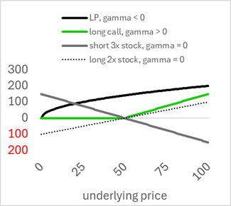
The Black-Scholes pricing model is the most famous equation in finance, and it has been studied and applied for over 50 years. It is not up for debate. They showed how any nonlinear payoff with non-zero gamma generates an expected non-zero payoff. Investors pay for long options because a positive gamma position's expected intrinsic value is greater than its current intrinsic value; investors get paid for short gamma positions because their expected liability is expected to grow over time. The value of this time value is called theta in the options literature.[Appendix: intuition on gamma expense]1
In the context of AMMs, we know the LP’s gamma,[Appendix: LP gamma]2 so with substitution we get
Note that this equation is a function of data that has nothing to do with MEV, adverse selection, or latency. Liquidity is straightforward to measure. The price and volatility of liquid coins like RUNE and BTC are determined worldwide on many exchanges, mainly off the blockchain. The peculiar MEV games on any DEX may be significant, but their effects are irrelevant to IL and usually focused on imprudently large retail trades.
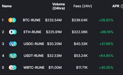
IL is universally recognized as an important cost, or at least a risk, for LPs. Yet, they are also universally ignored when presenting LP Annual Percentage Yields (APYs). When institutional research reports, blog posts, or podcasters mention an AMM protocol's profitability, they almost always refer to its revenues.
This expense is generally larger than fee revenue for large v3 AMMs, which is why they peaked four years ago in 2021. It's wishful thinking that not presenting the primary LP expense, usually greater than fee revenues, will become irrelevant if not reported.
Gamma expense is profoundly subtle, and appreciating it requires more than mere math knowledge. Unfortunately, most AMM protocols, like TC, do not understand it. This ignorance cost them severely in their Lenders program, but also in myriad other ways because it is so fundamental to any AMM. I cannot think of another field where its primary expense is universally neglected. It’s a cliche that you can’t manage what you do not measure, but it is no less accurate.
Bad Near-Death IL Lesson
TC initially offered its LPs IL protection insurance, reflecting its view that IL isn't material; it is just an academic concern about a hypothetical opportunity cost. It would be like offering park visitors insurance against Bigfoot attacks. In June 2022, Bancor defaulted on its IL insurance, and the protocol never recovered. After reaching $1.5B in 2021, Bancor fell to $100MM after the default and has languished there ever since.
Consider the price of BTC in RUNE from TC's inception in March 2021 through the end of its IL protection in November '23. The scale of the IL is arbitrary, but the point is that in this time window, intermediate non-zero IL was truly 'impermanent,' as it ended at zero.
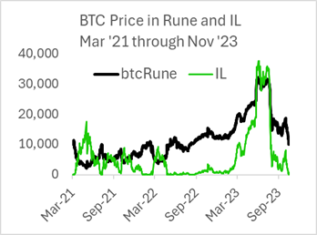
In August 2023, the Bitcoin/RUNE price reached a new high, creating a potential 17MM RUNE IL liability for TC. When the RUNE price rebounded and their IL protection liability became negligible, JPThor decided to end their IL protection, as at that point, it would not be a default, and they were not reneging on a large amount.
To JPThor, this proved that IL wasn't real; you just had to wait until the price reverted. TC dodged a bullet because, luckily, the LPs did not redeem their position and cash out on their IL protection. Their takeaway was that IL is important, but only because it exposes protocols to skittish LPs who do not have the patience to wait for the inevitable mean reversion; wiser traders just ignore it. This motivated their emphasis on single-sided liquidity, which has no IL risk. The problem was that single-sided liquidity is not liquidity; it was just easy to think so.
Poor Performance Metrics
At TC's mainnet launch in March 2021, they had over $100MM in the treasury for development, research, etc. They created many performance dashboards (see Thorchain , Thorcharts, Thoryield, ninerealms) and made much of their raw data available on flipside (table definitions here). It’s easy to report information, and the best way to obfuscate bad performance is simply to provide a lot of factual but ambiguously relevant data, like web search reports before Google introduced the idea of weighting results by importance.
Generally accepted accounting principles are boring but essential for any business. For investors, they tell where to allocate capital and are part of any process for estimating a company's value. For management, capital allocation is also essential. They also highlight businesses that either need fixing or exiting.
USD Denominated Returns
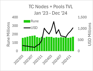
One major problem was that TC's total earnings were usually presented in USD. As TC runs on RUNE, presenting their earnings and TVL in USD obscures what is happening. The price of RUNE ranged from $1.00 to $10.00 in this period, so reported USD TVL ranged from $170MM to $1300MM, while RUNE TVL ranged only from 155MM to 185MM. As a prospective metric, as the average RUNE price was $3.8 over the past two years and $1.2 currently, the USD-denominated data will overstate any inference by over a factor of 3 in the future. Using RUNE in performance data generates a better picture than USD. The influence of the RUNE price on LP and validator returns is orthogonal to the profitability of the protocol.
60% of node and LP earnings were from minting RUNE
Since the protocol generated only $30MM a year in fees, using part of the $1B market cap to bootstrap early nodes and LPs seems reasonable. This would make TC look like it generated roughly $100MM/yr in profit and, given some look-back periods, $200MM a year (it’s common for influencer accounts pumping a protocol to use true-but-atypical data to make things look better). This helped mask weaknesses that needed attention. Inflating LP APYs caused insiders and outsiders to neglect fixing their AMM.
Streaming Swaps
Poor profitability reporting and a distracted focus on new flywheel products led to TC fumbling with the implementation of their streaming swaps feature.
Thorchain could extract a higher average liquidity fee by charging more for relatively larger trades while charging a significantly lower median liquidity fee versus standard flat fee AMMs that apply the same fee rate to every trade. Pulling in higher revenues from less cost-sensitive traders will subsidize lower fees for the rest and attract more traders overall.
Streaming swaps are similar to Time Weighted Average Price (TWAP) trades. They allow users to break a trade into pieces with less trade impact. This service is beneficial in tradfi, as many times one wants to trade more than the market can handle in one trade. For TC it was especially helpful because their unique fee was a function of the trade size, doubling the penalty for placing imprudently large orders. Such a tactic is easy to automate.
TC anticipated this would reduce their fee income by eliminating the high fees paid by ignorant or impatient traders who placed trades with high price impact and a high fee via their size-dependent slip fees. However, they thought the net benefit would be positive, as more whales would find TC an attractive alternative to bridges and CEXes.
TC reported average fees by averaging across transactions. A swap of 10 BTC with a high fee would be equally weighted with a swap of 0.01 BTC and a low fee. Arbitrageurs, who make only small trades to avoid paying extra fees, represent 60-70% of pool trading by volume and given the slip fee by transaction count. This method underestimated the weighted average fee rate. As these were presented on public dashboards, TC insiders presumably figured it was better marketing for TC.
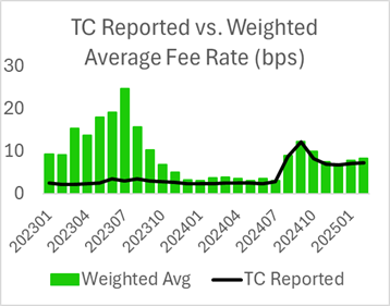
Unfortunately, this meant TC insiders were unaware their average fee rate fell from 16 bps from 3/2023 – 9/2023, to 3.5 bps from 1/2024 – 7/2024, a drastic decline. While volume increased, total fee revenue fell by half, and the variance in the latter period was double that of the earlier (and thus needed double the fee revenue).
In addition to TC's poor monitoring of effective fee rates, they were distracted by the two programs that led to their demise. Their Savers Vault was ramped up in October 2023 when the full effect of streaming swaps was finalized. Their Lenders program was introduced in March 2024. As the RUNE minting dominated total earnings, the drastic decline in fee revenue was not as conspicuous as it would have been.
Eventually, TC discovered a problem and added a fixed fee base of 6 basis points in August 2024. It took 9 months to rectify this problem, but it was apparent immediately if they had better performance metrics.
No IL in APYs
The leaders of the dominant AMM protocol, Uniswap, are fully aware of the LP’s primary expense, IL, which causes their most active AMM, the 5bp USDC-ETH pool, to continually lose money for its LPs. Not only do they not prominently display any IL information on current pools, but they have never published any broad data on the theta and fees generated by their most popular pools. Not measuring it will presumably help it get through the FUD until someone creates a magical hook that eliminates it. This is like a child closing his eyes so a monster cannot see him.
Like everyone else, TC presents the raw (feeRevenue + tokenInflation)/PoolValue APY, which is usually 20-60%. This made TC's base business look incredibly strong.
If you are the only AMM reporting net APYs, you will look bad, and as most AMM LPs don't understand the LP’s expense, however measured, being brutally honest may seem like bad marketing. The problem is that if you become an LP and continually see 60% returns and pull your money out a year later and find you have lost 25%, you are probably not coming back. This is relevant to all AMMs who have not regained their 2021 highs. Accurate reporting is good for businesses looking for repeat LPs.
Internal Sign LPs Were Never Generating 20%+ Returns
A clear sign that their LP APYs were wrong comes from TC's reporting on cumulative realized and unrealized P/L. Realized PnL was only calculated upon LP withdrawal, so monthly numbers reflected the life-cycle LP profitability of those who deposited last month or 24 months ago. This makes the monthly numbers virtually meaningless. This also will capture the IL assuming no hedge, which generates an extra standard error, as it reflects a singular price path that is not representative.
Nonetheless, if we combine the total realized LP pnl and the unrealized LP pnl up to the end of December 2024, we get an estimate of total LP performance drastically different than the standard 20-60% APYs presented. Below are TC's ETH and BTC pools, which represent about 50% of TC pool TVL.

Given their own data, which probably included token rewards, it's clear LPs weren't churning out the phenomenal APYs they would routinely present on various dashboards.
Another indicator that the LPs were not doing nearly as well as presented is their net deposits over 2023 and 2024. They were negative for both pools; LPs were leaving. LPs did not act like pool APYs were 20% +; if true, such a return would generate massive inflows.

The average age of an LP for these pools at the end of 2024 was 789 days. These are either hard-core TC supporters, delusional, or have lost their keys. They do not reflect a robust LP experience.
Intuition on the Gamma Expense
The essence of an option is from the non-zero gamma in the payoff state, which is also called convexity or nonlinearity, a payoff that is a nonlinear function of some underlying price. This cost is independent of any transaction costs involved in hedging via the bid-ask, fees, or price impact. However, hedging is desirable because it reduces the required capital as less cushion is needed for extreme drawdowns. In many cases, the risk can be virtually eliminated via the law of large numbers, but the expected benefit or cost of gamma remains unchanged.
The nice thing about option theory is that you can prove things in many different ways. This is true for most mathematically derived results, such as how there are 17 ways to prove the Pythagorean theorem. The benefit of additional proofs is that, given that our minds are different, one proof might appear more intuitive than the others for quirky reasons.
The simplest way to intuit gamma is a model that involves only algebra instead of stochastic differential equations. The binomial option pricing model (Cox, Ross, Rubinstein 1977) presents a riskless portfolio using a combination of a stock, bond, and option to a simple tree of states.
For example, assume a call with a strike of 100 and an initial stock price of 100. The underlying stock will go up or down by 10%, and the riskless rate is zero. If the stock goes up 10%, the call value is 10; if the stock goes down, the call is worthless. The portfolio can be perfectly hedged by a stock position equal to the call's delta. In the binomial model, you can calculate the hedge exactly with some simple algebra
plugging in for the specific parameters in our example, we have
Given a delta of 0.524, this implies the call writer hedges by going long this amount of stock. This portfolio generates the same payoff whatever happens, -4.76.
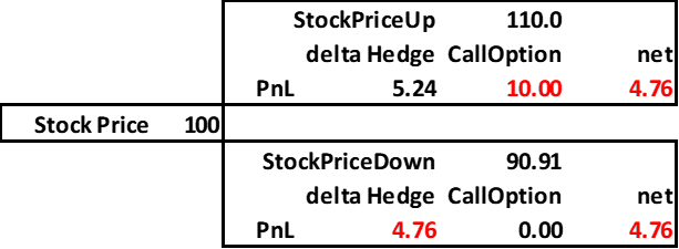
This shows how hedging turns the option payoff into a risk-free position. Further, note that the call value is the same using either the binomial model or present valuing the expected value of the payoff. As the interest rate is zero, the probability times the payoff is the discounted expected value.
Thus, one can sell the option and accept the risk liability of 10 or zero, where 10 has a 47.6% chance of happening, or hedge the option and pay 4.76 in the next period regardless.
A profound implication of the simple one-period binomial option is that if you were to write an option and see over a year that its cost was zero, this would tell you little about its initial true value, like rolling a die 3 times to estimate its probability of getting a six. Many IL commentators highlight a specific period where prices ended up where they started, and then note that the secret to good LP management is not exiting. This logical fallacy is so apparent that I have trouble framing the issue in a way that a person who thinks that way would appreciate, like thinking of how to explain the concept of 42 to a tribesman whose language for all numbers above 2 is ‘many.’
As the number of periods in the model goes to infinity and the time-step to zero, the binomial tree applied to the log of stock prices converges in distribution to the continuous geometric Brownian motion used in Black-Scholes.
The option price in the binomial model is computed using risk-neutral expectations:
As the underlying asset follows the same distribution as in Black-Scholes, this implies the Binomial model asymptotically equals the Black-Scholes formula, and can be applied to calculate option values as well as various Greeks.
How Black-Scholes estimated theta
The Black-Scholes proof was based on
Assuming stock prices follow geometric Brownian motion
Defining an option value as a function of price and time to maturity
Boundary condition for the option value at maturity
Constructing a risk-free portfolio containing the option and its hedge
A hedged portfolio with nonlinear derivative V(p) hedged is riskless
\(risklessPortfolio = V(option) - p \cdot hedge\)where
\(hedge = \Delta = delta = - \frac{{\partial V(option)}}{{\partial p}}\)Assuming arbitrage implies a risk-free portfolio, such as the hedged option position, has a zero profit
They apply Ito's Lemma to the portfolio value and derive the Black-Scholes partial differential equation (PDE). This can be used to solve not only for the option value but its many 'Greeks,' such as delta, gamma, theta, rho, etc.
The B-S PDE says that time decay plus the gamma payoff on the LHS of the equation equals the risk-free return on the capital used to create the hedged portfolio (note the interest rate r on the RHS). If interest rates are zero, the time decay or theta is equal to the negative of the messy term with a second derivative, denoted gamma. This is because, in equilibrium, the expected value of this position is zero; the time decay—dV/dt, theta—has to offset the gamma expense in equilibrium. The essence of an option is that this term is non-zero, reflecting the curvature, or non-zero gamma, in the portfolio's value.
For unrestricted range LPs, their value is
Thus, the gamma for a constant product AMM is:
Substituting this into the B-S theta equation gives us